What is Explainable Monte Carlo?
A late evening. You set up the model and simulated it at least a dozen times. A few mistakes are caught on the way. A few assumptions are challenged. The next step is to change several inputs at a time and see how it affects the results. Lots of iterations are ahead. There are already a few suspects that curiously change the model behaviour. Next morning brings some fresh ideas on what other model configurations can be checked. The manual what-if marathon continues.
Sounds familiar?
Many decision professionals confess to doing exactly that. The only situation that allows a quicker turnaround is when new models are structurally the same and hold no surprises.
That what-if marathon that iterates through the effects of multiple combinations of inputs on the output has already been automated for predictive machine learning (check SHAP). The field was coined as Explainable AI or XAI. Now it’s time for Monte Carlo simulation to have everyday tools that make it explainable.
What is explainable Monte Carlo?
Strictly speaking, it is a family of methods that bring transparency and interpretability to traditional Monte Carlo simulations. More practically, it translates the Monte Carlo evaluation into actionable information, as in: what needs to happen to land in the desired output range. The explainability enables several insights (more about each right after the list):
- Which inputs contribute to the variation of the output? [input importance]
- How do combinations of inputs map onto the distribution of the output? [input-output mapping]
- How does the importance of inputs change across the model space? [regional sensitivity profiles]
- Which inputs split the simulation into the most distinct sensitivity profiles? [heterogeneity]
1. Input importance
Input importance is the most familiar concept. Tornado diagrams and spider charts for one-at-a-time sensitivity analysis have been used for decades. The same old criticism, that such analysis fails to capture interactions and nothing in the world changes in isolation, has been resolved by the academic field of global sensitivity analysis. A plethora of methods developed in only a couple of decades [1] embraces almost every type of mathematics possible [2]. One intuitive way is to compute a portion of output’s variance that an input explains, an idea developed by Ilya Sobol’, a founding scholar of the field [3]. Modern improvements wrap that idea into an efficient computation algorithm that allows lifting all original constraints [4].
Having a number on the input importance is convenient. It focuses attention where it matters, highlighting which assumptions require more digging and (if that’s the best we know) which factors are an unignorable force.
But is it enough?
Does knowing that, for example, Price and Volume are the most important inputs give enough actionable information? Don’t we want to know what combinations of Price and Volume would lead to the attractive output range?
2. Input-output mapping
Matching inputs with outputs in a Monte Carlo simulation is like asking myriads of what-if questions simultaneously. But multidimensional visualization is a hard task. Imagine visualizing an entire input-output dataset with let’s say 10 inputs and 1000 simulation runs. What a mess that would be. Losing information is inevitable. The question becomes, how to preserve what matters. Here is how:
Step #1 - use already computed sensitivity indices to brush off non-important inputs and convert the multidimensional problem to a fewer-dimensional one.
Step #2 - instead of mapping each value, map the range:
- break the ranges of important inputs into states (Price: low, high),
- combine states into multi-variable scenarios (think low-Price && low-Volume, high Price && low Volume...), and
- use smart color-coding for those scenarios to tease out the patterns: the states of the most influential variable get distinct colors, other subdivisions - shades of it. The example below will make it vividly clear.
Step #3 - choose your visualization type
- A histogram, with scenarios stacked on top of each other.
- A box plot, with a box for each scenario
- A simple scatterplot, color-coded accordingly
- Or a combination of these.
That’s roughly the simulation decomposition idea [5]. The distribution of the output, otherwise usually shown in a single color, will suddenly show what was responsible for producing different portions of it. Questions such as these can be answered: What needs to happen to get to the high output? Is there another way to get there? (usually there is).
You might think: “I don’t need visualization to know that high Profit was produced by high Price and high Volume”. I’d answer: your model is rarely defined by a single arithmetical operation that can be reduced to such a simple linear conclusion. Many models, even simple at a glance, produce nonlinear and non-intuitive effects [5]. Various interactions, hiding behind the same sensitivity index, can produce an on and off effect, flip the direction of influence, or intensify the magnitude of an effect. Each case would imply a different decision recommendation.
3. Regional sensitivity profiles
We now know what inputs matter and how they drive the output. Is there anything left to learn about a simulation? Yes, there might be. Simulation decomposition intentionally focuses on inputs that are important globally. What if there is an input that appears not important on average but dominates in a small section of a model (for example, only low values of the output, or a single scenario, or a certain range of some input variable)?
The way to catch it is to look at regional sensitivity profiles, in other words, calculating the same sensitivity indices, but for portions of the simulation [6]. By the way, this is also a convenient way to see how different scenarios are if there is a scenario variable, which lets you skip running several simulations separately.
But if sensitivity profiles can potentially change across regions of an output and any (of many) inputs, is there a way to quickly spot which variables deserve attention and which can be safely neglected? Yes!
4. Heterogeneity
A convenient measure to detect a changing sensitivity profile is a heterogeneity index [7]. Zero means a stable sensitivity profile. Higher values mean something is happening and it’s worth having a look.
The idea behind the heterogeneity index is very simple: take a variable,
- split it into regions (quantiles or unique values for discrete variables),
- compute sensitivity indices for each region,
- compute the distance between each pair of regional sensitivity profiles, and
- take the average of these distances.
This way, each input and output in the model gets a number bounded between 0 and 1, which tells us whether the regions of that particular variable have similar or changing sensitivity profiles. If all heterogeneity indices are near zero, the global sensitivity indices can safely be trusted.
Enough of theory, let’s have a look at how it works.
Example
Let’s take something simple enough so that all the weirdness in the model would be fairly obvious.
Suppose there is a 45% chance to win a contract with uncertain, but more favourable price than the spot price. Uncertain volume is modelled with a stochastic process. Costs include an upfront investment, a unit cost, and fixed costs. The model computes the project value (NPV) over a 5-year time horizon. Here are all the numeric details:
| Variable | Value distribution |
|---|---|
| Contract won | Bernoulli(0.45) |
| Spot price, EUR/unit | Triangular(7.2, 8.4, 9.8) |
| Contract price, EUR/unit | Pert(10, 11, 12.4) |
| Unit cost, EUR/unit | Uniform(9, 10) |
| Fixed cost per year (thousand EUR) | 50 |
| Initial investment (thousand EUR) | Pert(80, 100, 140) |
| Discount rate (WACC) | Uniform(0.07, 0.1) |
| Volume, thousand units/year | GBM(start 100, drift 0.05, volatility 0.35) |
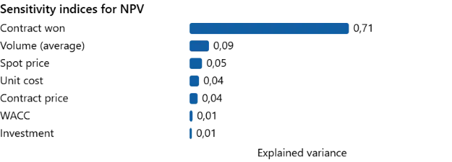
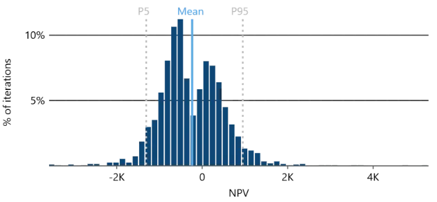
Simulating a model like this returns a funny bimodal distribution. As is not hard to guess, the two peaks correspond to the two scenarios with different prices. Sensitivity indices confirm our conjecture, revealing that over 70% of NPV variance is explained by whether the contract is won or not. A decision recommendation based on this would have been: invest if the contract is won.
Here the analysis of Monte Carlo simulation results usually ends. But explainable Monte Carlo digs further.
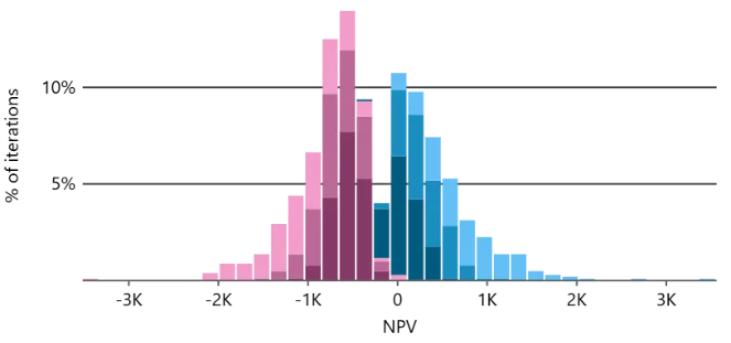
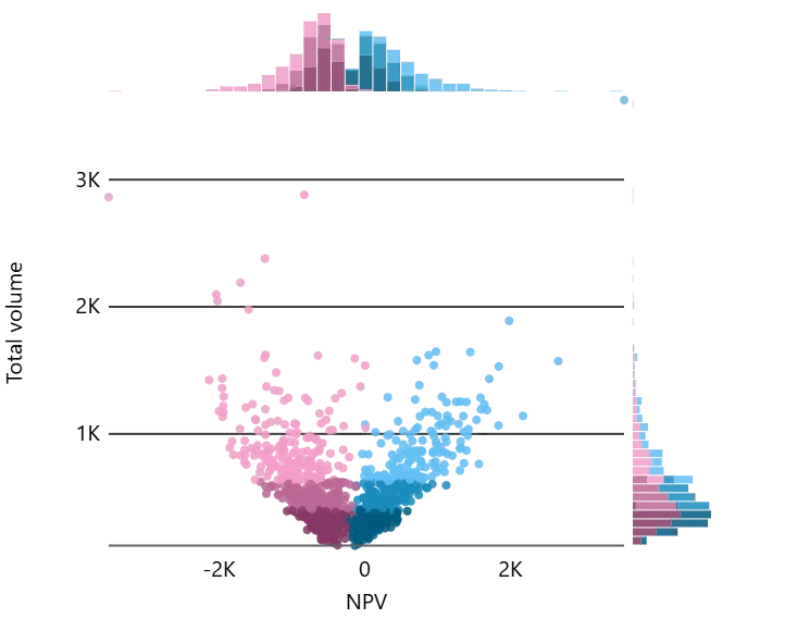
How do the main drivers, Contract won and Volume (average), map onto the NPV distribution? Here is how.
Multiple insights can be derived from this visual.
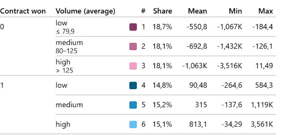
- Yes, the two peaks are attributed to the contract winning scenario: the right one (blue) enjoys the higher contract prices, the left one (pink) suffers from the lower spot prices.
- Interestingly, the effect of Volume flips its sign in the two peaks. The higher the volume the better when the contract is won (blue shades shift right from dark to light). But higher volume without the contract deteriorates the value (pink shades shift left from dark to light). Checking inputs’ assumptions reveals the simple explanation: spot prices are predominantly below unit cost.
- Winning the contract does not guarantee profitability. The combination of low volume and contract won (dark blue) partially leads to negative NPVs.
[If you want to see a case with a similar sign-flip effect that was not obvious even to the model owner, check the carbon footprint case from [5]].
Digging further, NPV gets a high heterogeneity index, prompting to look at the regional sensitivity indices:
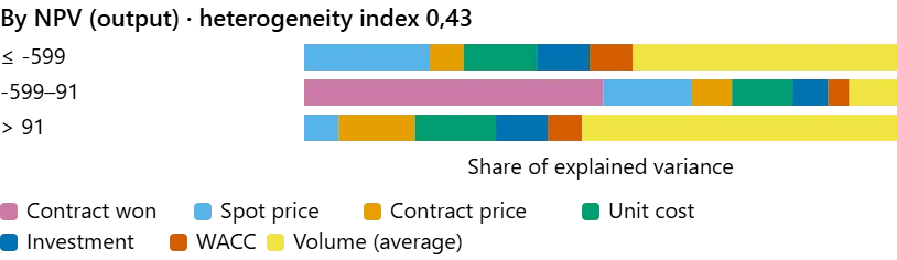
The middle region is dominated by Contract won, it’s what determines which peak we are in. The tail regions are, however, dominated by Volume, explaining about half of the NPV variance there. That’s where it hides its real power behind the low 9% global sensitivity index.
A more nuanced decision recommendation would then be: Make sure you win the contract and then push the volume. Otherwise abort.
P.S. The two peaks of this case made it into the Explainable Monte Carlo logo.
P.P.S. Explainable Monte Carlo methods and tools are developed with true passion 🩷🩵, visible even in its analytics:
References
[1] Tarantola, S., Ferretti, F., Piano, S. L., Kozlova, M., Lachi, A., Rosati, R., ... & Saltelli, A. (2024). An annotated timeline of sensitivity analysis. Environmental Modelling & Software, 174, 105977.
[2] Saltelli, A., Ratto, M., Andres, T., Campolongo, F., Cariboni, J., Gatelli, D., ... & Tarantola, S. (2008). Global sensitivity analysis: the primer. John Wiley & Sons.
[3] Sobol, I. M. (1993). Sensitivity estimates for nonlinear mathematical models. Math. Model. Comput. Exp., 1(4), 407–414.
[4] Kozlova, M., Ahola, A., Roy, P. T., & Yeomans, J. S. (2025). Simple binning algorithm and SimDec visualization for comprehensive sensitivity analysis of complex computational models. Journal of Environmental Informatics Letters, 13(1), 38–56. doi.org/10.3808/jeil.202400149
[5] Kozlova, M., Moss, R. J., Yeomans, J. S., & Caers, J. (2024). Uncovering heterogeneous effects in computational models for sustainable decision-making. Environmental Modelling & Software, 171, 105898. doi.org/10.1016/j.envsoft.2023.105898
[6] Helo, J., Kozlova, M., Roy, P., & Yeomans, J. S. (2026). Regional Variance-Based Sensitivity Analysis and a Study of Regional Equifinality. Risk Analysis, 46(10), e70346. doi.org/10.1111/risa.70346
[7] Kozlova, M., Helo, J., Roy, P. T., Yeomans, J. S., & Saltelli, A. (2026). Beyond Global Importance: A Heterogeneity Index for Sensitivity Analysis. arXiv preprint arXiv:2610.31008. arxiv.org/abs/2610.31008
More papers, the open-access SimDec book and the open-source packages are on the Resources page.